Plot cherry blossom bloom statuses

This vignette demonstrates how to use the bbggplots package to visualize the bloom statuses of cherry trees in the Brooklyn Botanic Garden. We will use custom SVG icons to represent different bloom stages and plot them on a map of the garden.

This effectively is the code behind the plot_map() function, but here we will show how to do it step by step, and how to customize the plot further if desired.

library(bbggplots)
library(dplyr)
#> 
#> Attaching package: 'dplyr'
#> The following objects are masked from 'package:stats':
#> 
#>     filter, lag
#> The following objects are masked from 'package:base':
#> 
#>     intersect, setdiff, setequal, union
library(ggplot2)
library(ggsvg)
library(ggpubr)

Each of the bloom stages (prebloom, first bloom, peak bloom, post bloom) has a corresponding SVG icon included in the package. We will read these SVG files into R and store them in a data frame for easy access.

firstbloom_svg <-
    system.file("extdata", "cherry-firstbloom.svg", package="bbggplots") |>
    readLines(warn = FALSE) |>
    paste(collapse = "\n")
peakbloom_svg <-
    system.file("extdata", "cherry-peakbloom.svg", package="bbggplots") |>
    readLines(warn = FALSE) |>
    paste(collapse = "\n")
postbloom_svg <-
    system.file("extdata", "cherry-postbloom.svg", package="bbggplots") |>
    readLines(warn = FALSE) |>
    paste(collapse = "\n")
prebloom_svg <-
    system.file("extdata", "cherry-prebloom.svg", package="bbggplots") |>
    readLines(warn = FALSE) |>
    paste(collapse = "\n")
bg <-
    system.file("extdata", "cherrymap.png", package="bbggplots") |>
    png::readPNG()

Now, we will create a data frame that maps each bloom stage to its corresponding SVG icon. This will allow us to easily merge this information with our tree data later on.

icons_df <- data.frame(
  bloom = c('Prebloom', 'First Bloom', 'Peak Bloom', 'Post Bloom'),
  svg  = c( prebloom_svg, firstbloom_svg, peakbloom_svg, postbloom_svg),
  stringsAsFactors = FALSE
)

And then finally, we can create the plot by filtering the data for a specific date, merging it with the tree positions and the icons, and then plotting it using ggplot2 with the background image of the garden map.

p_size <- 5
bg_dim <- dim(bg)
bbgdata |>
    filter(date == "2025-04-14") |>
    mutate(id = as.character(id)) |>
    left_join(treepositions, by = join_by(tree == tree, id == id)) |>
    mutate(
        x = (left / 100 * bg_dim[2]) + p_size,
        y = (-top / 100 * bg_dim[1]) - p_size
    ) |>
    merge(icons_df) |>
    ggplot() +
    background_image(bg) +
    geom_point_svg(
        aes(x = x, y = y, svg = I(svg)),
        size = p_size
    ) + 
    scale_x_continuous(
        expand = c(0, 0),
        limits = c(0, 550)
    ) +
    scale_y_continuous(
        expand = c(0, 0),
        limits = c(0, -498)
    ) +
    # Maintain 1:1 ratio and allow drawing outside limits
    coord_fixed(clip = "off") +
    theme_minimal()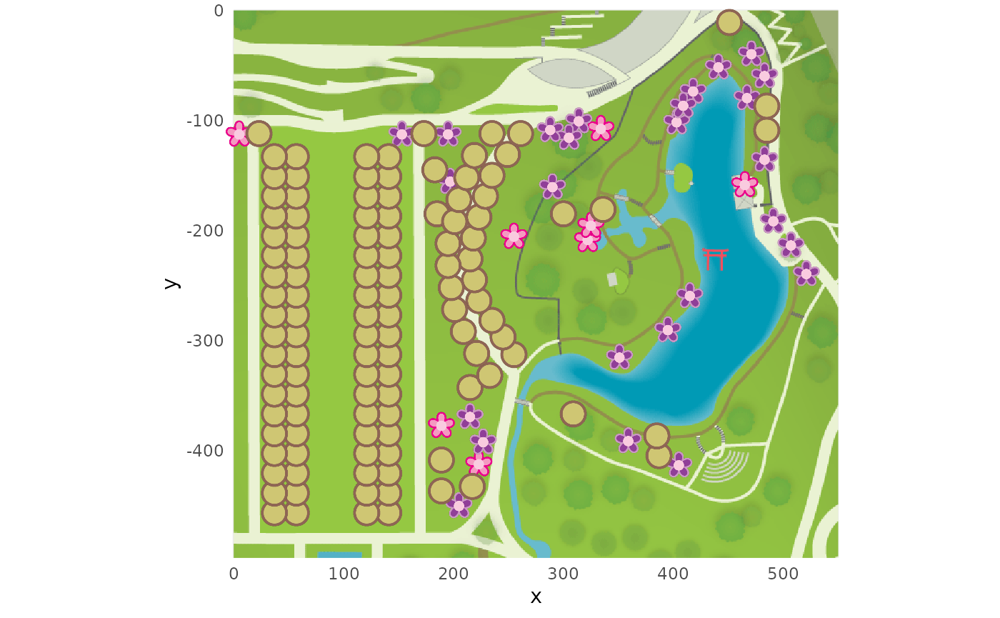

sessionInfo()
#> R version 4.6.0 (2026-04-24)
#> Platform: x86_64-pc-linux-gnu
#> Running under: Ubuntu 24.04.4 LTS
#> 
#> Matrix products: default
#> BLAS:   /usr/lib/x86_64-linux-gnu/openblas-pthread/libblas.so.3 
#> LAPACK: /usr/lib/x86_64-linux-gnu/openblas-pthread/libopenblasp-r0.3.26.so;  LAPACK version 3.12.0
#> 
#> locale:
#>  [1] LC_CTYPE=C.UTF-8       LC_NUMERIC=C           LC_TIME=C.UTF-8       
#>  [4] LC_COLLATE=C.UTF-8     LC_MONETARY=C.UTF-8    LC_MESSAGES=C.UTF-8   
#>  [7] LC_PAPER=C.UTF-8       LC_NAME=C              LC_ADDRESS=C          
#> [10] LC_TELEPHONE=C         LC_MEASUREMENT=C.UTF-8 LC_IDENTIFICATION=C   
#> 
#> time zone: UTC
#> tzcode source: system (glibc)
#> 
#> attached base packages:
#> [1] stats     graphics  grDevices utils     datasets  methods   base     
#> 
#> other attached packages:
#> [1] ggpubr_0.6.3         ggsvg_0.1.13         ggplot2_4.0.3       
#> [4] dplyr_1.2.1          bbggplots_0.0.0.9000
#> 
#> loaded via a namespace (and not attached):
#>  [1] gtable_0.3.6       jsonlite_2.0.0     compiler_4.6.0     ggsignif_0.6.4    
#>  [5] tidyselect_1.2.1   stringr_1.6.0      rsvg_2.7.0         tidyr_1.3.2       
#>  [9] jquerylib_0.1.4    png_0.1-9          systemfonts_1.3.2  scales_1.4.0      
#> [13] textshaping_1.0.5  yaml_2.3.12        fastmap_1.2.0      R6_2.6.1          
#> [17] labeling_0.4.3     generics_0.1.4     Formula_1.2-5      knitr_1.51        
#> [21] backports_1.5.1    tibble_3.3.1       car_3.1-5          desc_1.4.3        
#> [25] bslib_0.10.0       pillar_1.11.1      RColorBrewer_1.1-3 rlang_1.2.0       
#> [29] stringi_1.8.7      broom_1.0.12       cachem_1.1.0       xfun_0.57         
#> [33] fs_2.1.0           sass_0.4.10        S7_0.2.2           cli_3.6.6         
#> [37] pkgdown_2.2.0      withr_3.0.2        magrittr_2.0.5     digest_0.6.39     
#> [41] grid_4.6.0         lifecycle_1.0.5    vctrs_0.7.3        rstatix_0.7.3     
#> [45] evaluate_1.0.5     glue_1.8.1         farver_2.1.2       ragg_1.5.2        
#> [49] abind_1.4-8        carData_3.0-6      rmarkdown_2.31     purrr_1.2.2       
#> [53] tools_4.6.0        pkgconfig_2.0.3    htmltools_0.5.9

Eric Leung